-
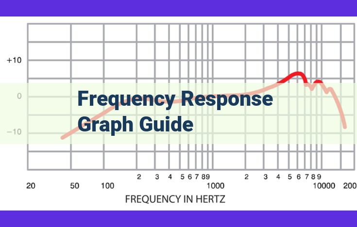
Introduction to Frequency Response Graphs:
These graphs depict the behavior of electronic circuits over various frequencies. -
Bode and Nyquist Plots:
Bode plots display gain and phase, while Nyquist plots provide insight into stability and performance. -
Key Parameters:
Gain affects signal amplitude, phase influences time shift, cutoff frequency separates gain and phase regions, while resonance frequency indicates maximum phase shift and gain. Damping ratio controls oscillations, and rise time, overshoot, and settling time measure signal response.
- Explain the purpose and significance of frequency response graphs.
In the realm of electronics and audio systems, frequency response graphs serve as invaluable tools, providing a comprehensive insight into the behavior and characteristics of a system. They unveil the intricate relationship between input frequencies and the corresponding output signals, offering a deeper understanding of how devices amplify, filter, and process signals. These graphs empower engineers, technicians, and audio enthusiasts alike with the knowledge to design and optimize systems for specific applications.
At their core, frequency response graphs are graphical representations that depict the gain and phase response of a system over a range of frequencies. Gain, measured in decibels (dB), indicates the amplification or attenuation of signal strength, while phase, measured in degrees, reveals the time delay or shift between input and output signals. By examining these graphs, we can identify key features such as cutoff frequency, resonance frequency, and damping ratio, which provide insights into the system’s performance and limitations.
Bode Plot: A Comprehensive Overview
- Describe the components of a Bode plot, including gain, phase, and cutoff frequency.
- Discuss how Bode plots compare to Nyquist plots.
Bode Plot: A Comprehensive Overview
Bode plots, named after the renowned electrical engineer Hendrik Bode, are essential tools for analyzing the frequency response of dynamic systems. These graphical representations depict how a system’s gain and phase change over a range of frequencies.
At the heart of a Bode plot lies the gain curve, which represents the ratio of the output signal’s amplitude to the input signal’s amplitude. The phase curve, on the other hand, shows the time delay or phase shift between the input and output signals.
One of the key parameters in a Bode plot is the cutoff frequency, which marks the point where the gain curve begins to roll off. This frequency is crucial in determining the bandwidth of the system, which is the range of frequencies over which the system can amplify signals effectively.
Bode plots provide a wealth of information about a system’s behavior. By observing the gain and phase curves, engineers can assess system stability, identify resonant frequencies, and predict transient responses. They can also compare different designs and optimize systems for specific performance requirements.
Moreover, Bode plots often serve as a bridge between theoretical analysis and practical measurements. Engineers can measure the frequency response of a system experimentally and then compare the results with the Bode plot predicted by the system’s model. This comparison helps validate the model and provides insights into the system’s actual behavior.
In contrast to Nyquist plots, which depict the system’s frequency response in the complex plane, Bode plots present the gain and phase as separate curves on a logarithmic scale. This simpler representation makes Bode plots more accessible and intuitive for many applications.
Nyquist Plot: Exploring Stability and Performance
In the realm of frequency response analysis, the Nyquist plot stands as a powerful tool used by engineers to assess the stability and performance of systems. It complements the Bode plot, offering a distinct perspective that unveils valuable insights into a system’s behavior.
Elements of a Nyquist Plot:
A Nyquist plot, like its counterpart, the Bode plot, consists of two key components:
- Gain: This parameter represents the amplification of the system’s output signal relative to its input. On the Nyquist plot, it is depicted as the distance from the origin to a given point.
- Phase: This attribute indicates the time shift between the input and output signals. It is represented by the angle between the line connecting the origin to a given point and the horizontal axis.
Similarities and Differences with Bode Plot:
While Nyquist and Bode plots share the common purpose of visualizing a system’s frequency response, they exhibit distinct differences:
- Format: A Nyquist plot is a parametric plot, displaying gain and phase as a single curve, while a Bode plot comprises two separate plots: one for gain and one for phase.
- Dimensionality: Nyquist plots are typically presented in a two-dimensional plane, whereas Bode plots are three-dimensional due to the inclusion of frequency as a variable.
- Orientation: The Nyquist plot is drawn in the complex plane, with the real part of the frequency response on the horizontal axis and the imaginary part on the vertical axis.
Exploring Stability:
The Nyquist plot plays a crucial role in determining the stability of a system. By inspecting the plot, engineers can identify the presence of encirclements around the critical point (-1,0). Each encirclement corresponds to a pair of complex conjugate poles that lie in the right half-plane, indicating an unstable system.
Enhancing Performance:
Beyond assessing stability, the Nyquist plot provides valuable information for optimizing system performance. By analyzing the plot’s shape and characteristics, engineers can identify potential resonance frequencies and adjust system parameters to mitigate unwanted oscillations and improve overall system behavior.
**Gain: The Signal Strength Amplifier**
In the realm of frequency response graphs, gain plays a pivotal role in amplifying the strength of signals, like a conductor orchestrating a symphony. It represents the ratio of the output signal to the input signal, determining the overall amplitude of the amplified signal.
Gain has a profound impact on the signal’s amplitude, akin to a volume knob controlling the loudness of a stereo. By increasing the gain, we amplify the signal, making it louder and more pronounced. Conversely, reducing the gain dampens the signal, reducing its amplitude and making it quieter.
The relationship between gain, phase, and cutoff frequency is a delicate dance. Gain primarily affects the amplitude of the signal, while phase represents a time shift and cutoff frequency determines the range of frequencies that are amplified. Together, they form a trinity that shapes the overall behavior of the system.
Phase: The Time-Shifted Signals
Phase is a crucial aspect of frequency response graphs, as it measures the time shift between the input and output signals. It’s expressed in degrees or radians and plays a significant role in understanding how signals behave in a system.
Imagine a musical instrument like a guitar. When you pluck a string, the vibration of the string creates a sound wave that travels through the air. This sound wave has both amplitude (volume) and phase (timing).
If you pluck two strings simultaneously, they may vibrate at the same frequency but have different phases. This difference in phase determines whether the sound waves will reinforce or cancel each other out. When the peaks of the waves align, they enhance each other, resulting in a louder sound. When the troughs of the waves align, they cancel each other out, creating a quieter sound.
In electrical systems, phase is equally important. Consider a circuit with an amplifier. When an input signal is applied, the amplifier may not only amplify its amplitude but also shift its phase. This phase shift affects the timing of the output signal.
For example, in a resonant circuit, the phase shift between the input and output signals is directly related to the resonance frequency. At resonance, the phase shift is zero, meaning the input and output signals are perfectly aligned. This alignment leads to maximum energy transfer and the highest possible amplitude in the output signal.
Understanding phase is crucial for analyzing and designing circuits because it can affect factors such as stability, bandwidth, and distortion. By mastering this concept, you can delve deeper into the fascinating world of frequency response graphs and gain a profound understanding of how signals behave in electrical systems.
Cutoff Frequency: The Grenze
In the realm of frequency response graphs, where signals dance and circuits interplay, lies the pivotal concept of cutoff frequency—a pivotal boundary that alters the very fate of signals. It’s a threshold where the signal’s strength wanes, the phase shifts, and the circuit’s response undergoes a metamorphosis.
Defining Cutoff Frequency
Envision a frequency response graph, a canvas upon which signals leave their imprint. Cutoff frequency is that pivotal point along the frequency axis where gain and phase undergo a dramatic transformation. It’s the demarcation between the high and low frequencies, where a signal’s influence wanes and its impact diminishes.
Influence on Gain and Phase
As frequencies approach and surpass the cutoff frequency, a noticeable shift occurs. Gain, the amplifier of signal strength, gradually diminishes, reducing the signal’s amplitude. Simultaneously, the signal’s phase—its temporal alignment—begins to lag, indicating a delay in its arrival.
Relationship to Resonance Frequency
Cutoff frequency shares an intimate relationship with resonance frequency, the point where a circuit’s response reaches its peak. As cutoff frequency increases, resonance frequency tends to decrease. This inverse correlation ensures that signals within a specific frequency band receive maximum amplification, while those beyond the cutoff frequency are attenuated.
By understanding cutoff frequency, engineers can design circuits that optimize signal transmission and minimize unwanted noise. It’s a crucial parameter that governs the performance and stability of electronic systems, shaping the flow of signals across the electronic landscape.
Resonance Frequency: The Peak of Excitation
Resonance frequency, a crucial parameter encountered in various engineering applications, unveils the fascinating behavior of systems when they are subjected to external forces. It represents the frequency at which a system is most responsive, exhibiting maximum amplitude oscillations.
Defining Resonance Frequency
Imagine a child on a swing. When you push the swing rhythmically at its resonance frequency, the swing reaches its highest oscillations. This is because the energy added by the rhythmic pushes matches the swing’s own frequency of oscillation, amplifying its motion. In electrical circuits and mechanical systems, resonance frequency plays a similar role, denoting the frequency where the system’s response is maximized.
Influence on Phase and Gain
As the frequency of an external force approaches the resonance frequency, the phase of the system’s response shifts. The phase is the time difference between the input and output signals. At resonance, the output signal is in phase with the input signal, while below resonance, it lags behind, and above resonance, it leads. The gain of the system, representing the ratio of output to input signal amplitude, also peaks at resonance frequency.
Damping Ratio’s Role
Damping ratio, a key factor in resonance frequency, controls how quickly oscillations decay after the external force is removed. A system with a high damping ratio will have less pronounced oscillations and a narrower resonance peak. Conversely, a low damping ratio will result in larger oscillations and a wider resonance peak.
In conclusion, resonance frequency is a vital concept that governs the response of systems to external forces. Understanding its influence on phase, gain, and the role of damping ratio is essential for analyzing and designing systems that operate near resonance.
Damping Ratio: Controlling Oscillations
In the world of signals and systems, stability and performance are paramount. One crucial factor that directly affects these attributes is the damping ratio, a parameter that elegantly controls oscillations within a system.
Defining Damping Ratio
The damping ratio, denoted by the Greek letter zeta (ζ), quantifies the ability of a system to dissipate energy during oscillations. It represents the level of damping or resistance present in the system. A damping ratio of zero indicates no damping, while higher values indicate increasing damping.
Impact on Resonance Frequency
Damping ratio significantly impacts the system’s resonance frequency, which is the frequency at which the system resonates or exhibits maximum oscillations. Higher damping ratios lead to lower resonance frequencies, effectively shifting the peak of excitation spectrum to the left.
Effect on Overshoot and Settling Time
Overshoot, the amount by which the system’s response exceeds its final steady-state value, is directly influenced by the damping ratio. Higher damping reduces overshoot, allowing the system to reach its intended level without excessive oscillations.
Settling time, the duration it takes for the system to stabilize within a specified tolerance, is also affected by the damping ratio. Higher damping ratios lead to shorter settling times, as the system reaches its final value more quickly and with less lingering oscillations.
Role in System Stability
The damping ratio plays a crucial role in determining the stability of a system. Systems with low damping ratios tend to oscillate excessively, potentially leading to instability and poor performance. Conversely, systems with high damping ratios exhibit controlled oscillations and achieve stability more rapidly.
The damping ratio is a fundamental concept in signal processing and control theory. It governs how a system dissipates energy during oscillations, affecting its stability, performance, and frequency response. By understanding the impact of damping ratio, engineers can optimize systems for precise and reliable operation.
Overshoot: Exceeding the Intended
When a system responds to an input, it often overshoots the desired output value before settling back to its intended destination. This phenomenon occurs when the system has insufficient damping, causing it to oscillate around the equilibrium point. The extent of overshoot is directly proportional to the damping ratio.
A low damping ratio results in significant overshoot because the system has less resistance to oscillations. This can lead to excessive колебаний, extending the settling time and potentially causing system instability. Conversely, a high damping ratio minimizes overshoot by increasing the damping force, reducing oscillations, and promoting faster settling.
Overshoot can have both positive and negative consequences. In some applications, a small amount of overshoot can be desirable, as it can provide a quick response. However, excessive overshoot can degrade performance, potentially leading to instability and even system damage.
Therefore, it is crucial to optimize the damping ratio to achieve the desired level of overshoot. A system with too little damping will experience excessive oscillations and overshoot, while a system with too much damping will settle slowly and may not respond quickly enough to changes in input. Finding the optimal balance is essential for ensuring system stability and performance.
Settling Time: Achieving Stability
In the realm of frequency response analysis, settling time emerges as a crucial parameter that governs the stability and performance of a system. Defined as the time it takes for a system’s output to reach and remain within a specified percentage (typically 2%) of its final steady-state value, settling time plays a pivotal role in ensuring system reliability.
The damping ratio exerts a profound influence on settling time. A lower damping ratio corresponds to a slower settling time, as the system oscillates more before reaching its final value. Conversely, a higher damping ratio leads to a faster settling time, resulting in a quicker response to changes in input.
Furthermore, overshoot significantly impacts settling time. Overshoot, characterized by the temporary overshooting of the final value before settling, is directly proportional to the damping ratio. A higher damping ratio minimizes overshoot, while a lower damping ratio allows for greater overshoot.
Relationship between Settling Time, Overshoot, and Rise Time
Settling time, overshoot, and rise time form an intricate triad of parameters that collectively shape a system’s response. Rise time, representing the time it takes for the output to reach a specified percentage of its final value (usually 10%), exhibits an inverse relationship with settling time. A faster rise time invariably leads to a shorter settling time.
In essence, settling time stands as a critical metric that measures the efficiency with which a system achieves stability after a change in input. By grasping the interplay between settling time, damping ratio, overshoot, and rise time, engineers and designers can optimize system performance, ensuring both responsiveness and reliability.
Rise Time: The Quickest Path
Understanding Rise Time
- Rise time measures how quickly a signal’s amplitude transitions from 10% to 90% of its final value.
- It represents the duration required for a signal to reach its intended operating level.
Rise Time and Settling Time
- Settling time is the period it takes for a signal to stabilize within a specified tolerance band around its final value.
- Rise time influences settling time because a faster rise time leads to:
- Lower overshoot, or smaller peaks of oscillation.
- Shorter settling time, as the signal reaches its steady-state faster.
Optimizing Rise Time and Settling Time
To minimize settling time and overshoot while achieving the desired system response, consider the following strategies:
-
Reducing Rise Time:
- Increasing the bandwidth of the system.
- Lowering the order of the system, which simplifies its response.
-
Optimizing Settling Time:
- Increasing the damping ratio reduces oscillations but can slightly increase rise time.
- Adjusting the loop gain or input signal frequency can fine-tune the settling time while considering rise time constraints.
Rise time plays a crucial role in system response by defining how quickly a signal reaches its operating level. It impacts settling time, overshoot, and system stability. By optimizing rise time and related parameters, engineers can ensure reliable signal performance and meet specific design constraints.