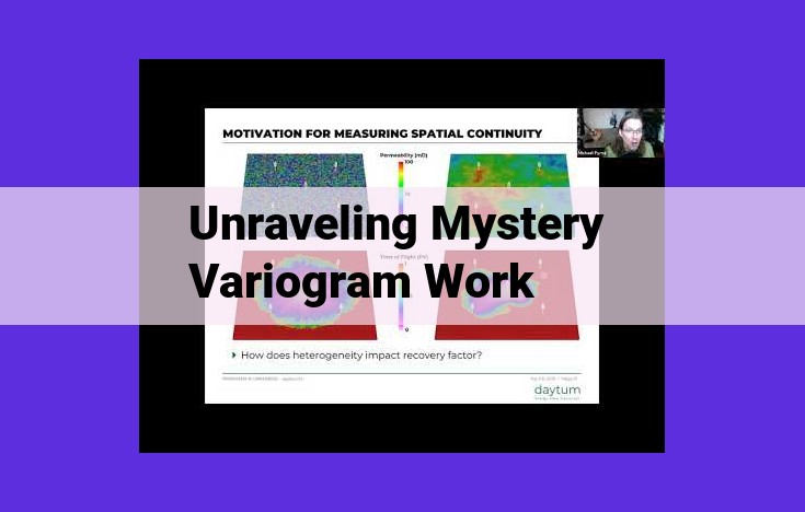
Unraveling mystery variogram work involves analyzing spatial variability through semivariance, which measures variance between data points over distance. A variogram plots semivariance against distance, revealing key characteristics like range (spatial influence), sill (total variability), nugget effect (local irregularities), and anisotropy (directional variations). These features provide insights into spatial structures and enable interpolation and modeling by understanding the scale, correlation, and directional dependencies of spatial processes.
Semivariance: Unveiling the Secrets of Spatial Variability
In the realm of spatial analysis, semivariance plays a pivotal role in deciphering the intricate tapestry of spatial variability. It’s a fundamental measure that quantifies how similar or dissimilar values are at different locations, providing a deep understanding of the patterns and relationships within spatial data.
Semivariance is calculated as half the expected squared difference between the values of two points separated by a specific distance. Intuitively, it represents the average squared difference between values at varying distances, offering insights into the degree of spatial heterogeneity. The smaller the semivariance, the more similar the values are at a given distance, indicating less spatial variability. Conversely, larger semivariance values suggest greater spatial heterogeneity.
Variograms: Painting the Canvas of Spatial Structure
Semivariance is the cornerstone upon which variograms are built. A variogram is a graphical representation of semivariance values plotted against the separation distance between pairs of data points. It’s akin to painting a picture of the spatial structure within the data.
Variograms exhibit a characteristic shape that reveals important characteristics of the spatial process:
- Range: The distance at which semivariance reaches a constant asymptote, indicating the limit of spatial dependence.
- Sill: The constant asymptotic value, representing the total variability in the data.
- Nugget Effect: The intercept of the variogram at a distance of zero, representing short-range variability due to measurement errors or microscale variations.
Nugget Effect: Capturing the Tiny Irregularities
The nugget effect captures the small-scale irregularities that cannot be explained by the spatial structure. It’s particularly important in environmental datasets, where factors like measurement errors, local topography, or biological heterogeneity can introduce a random noise component.
Range: Delineating the Zone of Influence
The range of a variogram defines the spatial extent of dependence or correlation. It indicates the distance beyond which values become independent of each other. This information is crucial for determining the appropriate scale of data sampling and interpolation.
Variogram: Unraveling the Mystery of Spatial Structure
In the realm of spatial analysis, the variogram emerges as a captivating tool for uncovering the hidden secrets of spatial data. It’s a graphical representation that unveils the intricate tapestry of spatial variability, helping us understand how data points are interconnected across space.
Plotting the Variogram
Envision a scatter plot with a twist. Instead of plotting data points against a linear axis, a variogram plots pairs of data points along the horizontal axis, representing the distance (or “lag”) between them. The vertical axis captures the difference between the values of these paired points. As we increase the lag distance, we effectively explore spatial variability at different scales.
Unveiling the Variogram’s Key Characteristics
This seemingly simple graph conceals a treasure trove of information:
- Range: This pivotal distance marks the threshold beyond which data points become spatially independent. It reveals the scale at which processes operate in the landscape.
- Sill: The sill represents the total variability present in the data. It indicates the maximum level of dissimilarity that can exist between data points.
- Nugget Effect: This enigmatic component captures short-range, random variability that cannot be explained by spatial processes. It often reflects measurement errors or microscale heterogeneity.
- Anisotropy: Variograms can sometimes exhibit directional variability, known as anisotropy. This fascinating trait suggests that spatial processes behave differently in different directions.
Implications for Spatial Analysis
The variogram serves as a guiding light for spatial analysis, illuminating the path towards:
- Spatial Sampling: The range of a variogram dictates the appropriate sampling interval for capturing spatial patterns accurately.
- Spatial Modeling: Variograms provide invaluable insights into the spatial structure of data, aiding in the development of accurate models that mimic real-world processes.
- Interpolation: Variograms guide interpolation algorithms, ensuring smooth and accurate predictions of values at unsampled locations.
Nugget Effect: Unveiling the Local Irregularities of Spatial Data
Beneath the seemingly smooth tapestry of spatial data lies a hidden layer of local irregularities. This concealed component, known as the nugget effect, holds significant importance in understanding the intricate nature of spatial phenomena.
Defining the Nugget Effect
The nugget effect represents the portion of spatial variability that occurs at distances too small to be detected by the sampling method. It signifies the abrupt variations or measurement errors that cannot be attributed to any discernible spatial structure.
Factors Contributing to the Nugget Effect
Several factors contribute to the nugget effect, including:
- Measurement errors: Imperfect instruments or sampling techniques can introduce random noise into the data, leading to a non-zero nugget effect.
- Microscale variability: Natural processes often exhibit fine-scale variations that fall below the resolution of the sampling method, resulting in a nugget effect.
- Spatial data aggregation: When data is aggregated from finer to coarser scales, small-scale variability can be obscured, increasing the nugget effect.
Significance in Spatial Analysis
The nugget effect plays a crucial role in spatial analysis by uncovering local, short-range variations that might otherwise remain hidden. It helps researchers:
- Identify measurement or sampling issues: A large nugget effect can indicate potential problems in data collection or processing.
- Estimate the accuracy of spatial interpolation: The nugget effect affects the prediction error of interpolation methods, necessitating its consideration in assessing the reliability of spatial predictions.
- Understand the underlying processes: The magnitude and shape of the nugget effect can provide insights into the nature of the underlying spatial phenomena, such as the presence of microscale processes or measurement limitations.
By deciphering the nugget effect, researchers gain a more comprehensive understanding of the spatial data they handle, allowing for more accurate interpretations, reliable predictions, and informed decision-making.
Range: Defining the Zone of Influence in Spatial Analysis
In the realm of spatial analysis, the range of a variogram plays a crucial role in understanding the spatial processes that shape our world. It’s like a boundary that defines the extent to which spatial features influence each other.
Imagine a vast landscape dotted with trees. A variogram can tell us how the height of one tree is related to the height of its neighbors. As we increase the distance between trees, the relationship weakens until it reaches a point where there’s no discernible correlation. This point of zero correlation marks the range of the variogram.
The range is a critical indicator of the scale at which spatial processes operate. For instance, a short range suggests that spatial features are highly localized, while a long range indicates that influences extend over greater distances. This knowledge is invaluable in designing sampling strategies and selecting appropriate analysis techniques.
For example, if we’re interested in studying the distribution of soil nutrients in a field, a variogram with a short range would suggest that soil samples should be collected at closely spaced intervals to capture the local variability. Conversely, if the range is long, a wider sampling spacing would be appropriate to avoid redundant data collection.
In a broader sense, understanding the range of a variogram helps us comprehend the underlying mechanisms that shape spatial patterns. It’s like a key that unlocks the hidden relationships that govern our environment and provides valuable insights for decision-making and resource management.
Sill: The Asymptote of Spatial Variability
When analyzing spatial data, the sill unveils crucial information about the total variability within a dataset. It represents the upper limit of the variogram, where spatial autocorrelation ceases to exist.
The sill reflects the aggregate variability of the dataset, incorporating both structural variability and random noise. Reaching the sill signifies that any further increase in distance does not contribute to the spatial dependence within the data.
Understanding the sill is paramount in variogram analysis. It helps determine the range (maximum distance of spatial autocorrelation) and partial sill (structural variability). By reaching the sill, we can identify the scale at which spatial processes stabilize, providing valuable insights into the underlying spatial patterns.
Partial Sill: Unveiling the Structural Variability
- Define partial sill and explain how it separates structural variability from the nugget effect.
- Discuss the use of partial sill in identifying different spatial components.
Unveiling the Structural Variability: The Partial Sill’s Story
In the realm of spatial analysis, understanding the intricate tapestry of data variability is the key to unlocking valuable insights into the world around us. This is where the partial sill, a hidden gem within the variogram, steps into the spotlight.
The partial sill is a subtler yet profound measure that unveils the true extent of structural variability hidden beneath the surface of the variogram. It deftly separates this structural variability from the nugget effect, a mischievous little anomaly that represents local irregularities and measurement uncertainties.
Think of the partial sill as a bridge, a conduit connecting the nugget effect to the sill, the plateau that signifies the dataset’s total variability. This bridge reveals the intricate dance of spatial patterns that unfold across varying distances.
By carefully examining the partial sill, we can discern different spatial components that contribute to the overall variability. It’s like a detective meticulously sifting through clues, unearthing the underlying mechanisms that shape the spatial landscape.
From the subtle dance of microscale variability to the sweeping grandeur of large-scale patterns, the partial sill offers a window into the intricate world of spatial processes. It guides us toward a deeper understanding of the forces that shape our environment, enabling us to make informed decisions and unravel the mysteries of our interconnected world.
Anisotropy: Unveiling Hidden Patterns in Spatial Data
In the realm of spatial analysis, anisotropy unveils a captivating aspect of spatial variability. It acknowledges that the patterns in your data may not be equal in all directions, like the ripples in a pond that spread differently based on the wind’s whims.
Imagine a field of sunflowers swaying gracefully. While they may appear uniform from afar, a closer look reveals subtle differences. Some bloom taller in the east-west direction, while others reach higher in the north-south direction. This directional variation is what we call anisotropy.
In variograms, the graphical representation of spatial variability, anisotropy manifests itself in the shape of the graph. Instead of a smooth, circular shape, anisotropic variograms exhibit elongation along specific axes. This elongation indicates that the spatial correlation is stronger in certain directions than others.
Understanding anisotropy is crucial for accurate spatial modeling and interpolation. Traditional methods that assume isotropic behavior may overlook these directional patterns, leading to errors in predicting values at unmeasured locations. By incorporating anisotropy into our models, we can capture the true complexity of our data and make more precise predictions.
For example, in environmental modeling, anisotropic variograms can help us understand the dispersal patterns of pollutants or the spread of invasive species. In resource exploration, they guide us in targeting areas with higher mineral concentrations or groundwater potential.
Embracing anisotropy enriches our understanding of spatial processes and empowers us to make informed decisions based on more accurate spatial data.
Cross-Variogram: Unveiling the Hidden Interconnections
Stepping into the realm of spatial analysis, one encounters a treasure trove of tools for understanding the intricate relationships that govern the world around us. Among these tools, variograms stand out as powerful instruments for unraveling the spatial structure lurking within data. While traditional variograms reveal the variance within a single variable, cross-variograms take this concept a step further, shedding light on the correlations between different variables.
Imagine a scientist studying the interplay between tree species and soil moisture. A cross-variogram can provide unparalleled insights by quantifying how the variance in tree species at different locations co-varies with the variance in soil moisture. This knowledge unveils the intricate dance between vegetation and hydrology, guiding conservation efforts and predicting ecosystem responses to environmental change.
Cross-variograms have proven indispensable in diverse fields ranging from ecology to geology. In agriculture, they help farmers optimize crop yields by understanding how soil properties influence plant growth patterns. In urban planning, they inform decisions on land use zoning by revealing the spatial correlations between traffic patterns and air pollution levels.
The beauty of cross-variograms lies in their ability to reveal complex spatial interactions that would otherwise remain hidden. They allow researchers and practitioners to uncover subtle patterns, identify underlying processes, and make informed decisions based on a deeper understanding of their data.